

Monte Carlo Capital Simulation
Traditional investment calculators project growth using a constant interest rate. However, real-world market returns fluctuate randomly. Firewire Analytics incorporates a Monte Carlo simulation engine (10,000 iterations) to evaluate plan resilience under volatility and Sequence of Returns Risk.
1. Why Monte Carlo Simulation?
Even if historical stock return averages $14\%$ per year, a portfolio might face negative returns during early withdrawal years (e.g. $-20\%$, $-15\%$). Withdrawing funds during market drops depletes capital much faster than deterministic models predict.
The Monte Carlo method simulates 10,000 independent future paths, capturing bull markets and market crashes.
2. Simulation Step Model
The simulation runs in yearly steps. At each step, every scenario draws an annual return $r_t$, capital $S_t$ is multiplied by $(1 + r_t)$, and only after that growth the year's net cash flow $C_t$ is added. Capital never goes below zero:
where:
- $S_t$ — portfolio capital at the start of year $t$;
- $r_t$ — the random annual return for that year;
- $C_t$ — net annual cash flow ($C_t = \text{Inflows} - \text{Outflows}$; an inflow or outflow counts in every year of its range, including the first and last);
- $\mu$ — expected return;
- $\sigma$ — annualized volatility;
- $Z_t \sim \mathcal{N}(0, 1)$ — standard normal random variable, independent for each year and scenario.
How $r_t$ is drawn depends on the calculator's “Distribution Type” switch:
- Normal (the default) — the annual return itself is normal: $r_t = \mu + \sigma \cdot Z_t$, i.e. $r_t \sim \mathcal{N}(\mu, \sigma^2)$. This is not Geometric Brownian Motion: the return is normal, not its logarithm.
- Lognormal — the logarithm of the annual growth factor is normal: $1 + r_t = \exp\left( \ln(1 + \mu) - \frac{\sigma^2}{2} + \sigma \cdot Z_t \right)$. The drift is $\ln(1 + \mu) - \sigma^2/2$, not $\mu - \sigma^2/2$, so the mean annual growth factor is exactly $1 + \mu$ and the return never falls below $-100\%$. This is a yearly (discrete) analogue of Geometric Brownian Motion.
- Risk-free — $r_t = \mu$ every year; all scenarios coincide and the result equals a constant-rate projection.
Because $C_t$ is added after growth, an inflow starts earning returns only from the following year, and a year's outflow does not reduce the capital that earns that same year's return. Once capital hits zero it stays at zero until later inflows replenish it.
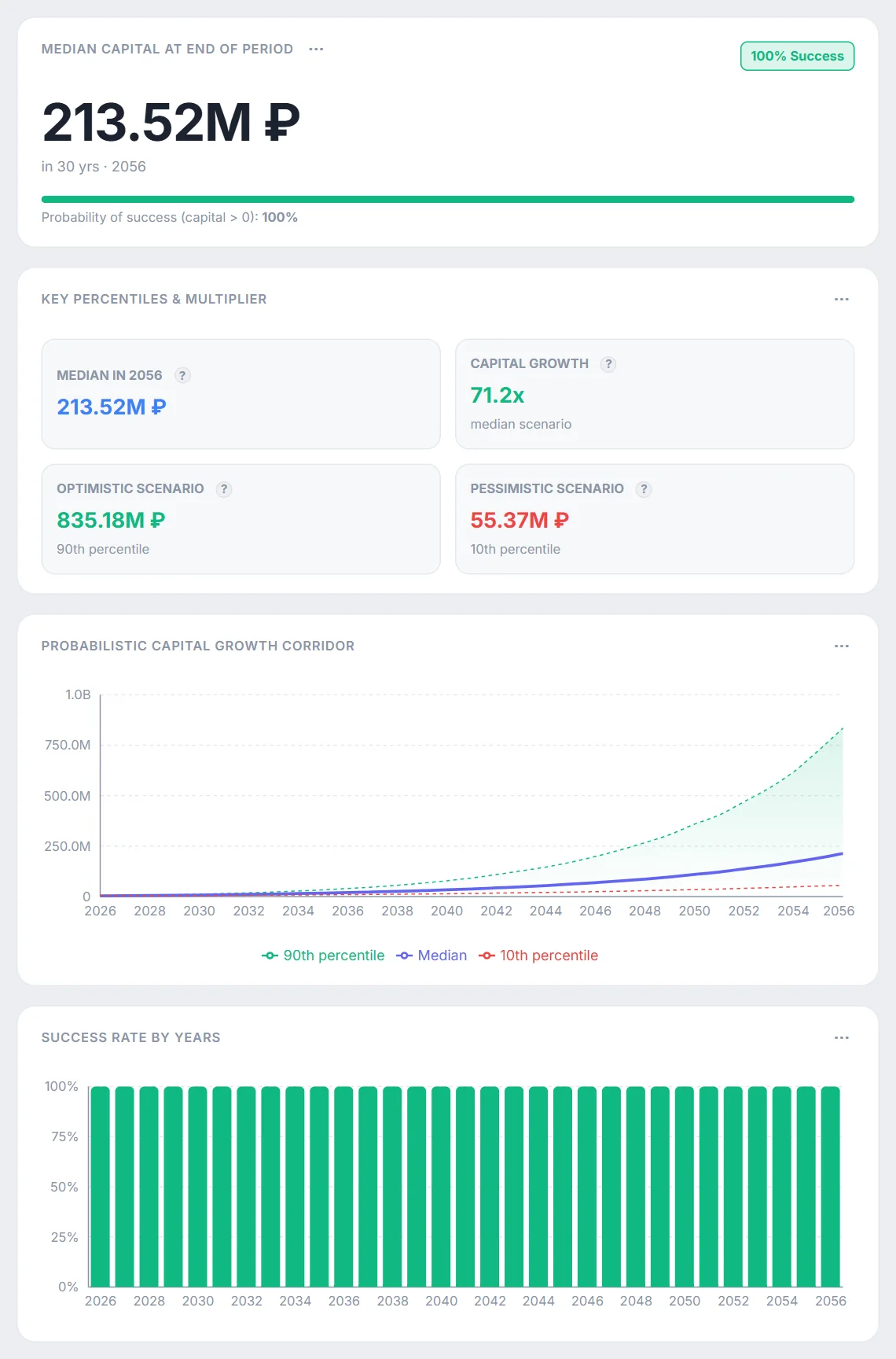
3. Scenario Percentiles ($P_{10}$, $P_{50}$, $P_{90}$)
- Median scenario ($P_{50}$) — $50\%$ of simulations performed better, $50\%$ worse.
- Optimistic scenario ($P_{90}$) — top $10\%$ quantile corresponding to strong bull markets.
- Conservative scenario ($P_{10}$) — bottom $10\%$ quantile representing severe early downturns.